1. Rainbow Classification
오늘은 무지개, 7가지 색을 인공지능을 통해 구분하는 시간입니다. 이는 이미 Label이 지정된 Supervised Learning이며 추가적으로 Neural Net(Multi Layer Perceptron)으로 구성했음을 미리 알려드립니다.
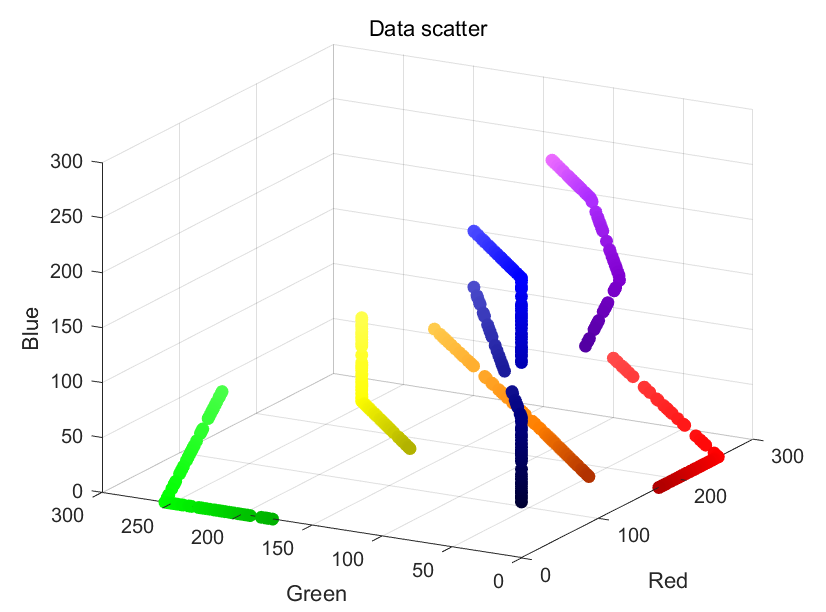
1.1. Definition 7 colors
7가지 색상에 대해서 코드를 정의합니다. 또한 label 은 학습과 결과에 대한 시각화를 위해 반드시 선언해줍니다.
1
2
3
4
5
6
7
8
9
10
11
12
clc, clear
rng('shuffle')
red = [255 0 0];
orange = [255 127 0];
yellow = [255 255 0];
green = [0 255 0];
blue = [0 0 255];
navy = [0 0 128];
purple = [160 32 240];

label = {'red' 'orange' 'yellow' 'green' 'blue' 'navy' 'purple'};
color = {red, orange, yellow, green, blue, navy, purple};
1.2. Check colors

분명 맥북에서는 파란색이었는데....글을 쓰는 이 모니터에선 색이 이상하다
plot을 통해 의도한 색상이 나왔는 지 확인합니다.
1
2
3
4
5
6
7
8
9
10
figure
for i=1:7
    subplot(2, 4, i)
    temp = color{i};
    hexStr = dec2hex(temp);
    str = strcat('#', hexStr(1,:), hexStr(2,:), hexStr(3,:));
    rectangle('Position', [0 0 1 1], 'FaceColor', str);
    xticks([])
    yticks([])
end
1.3. Select save directory
uigetdir은 UI를 통해 지정한 경로를 가져옵니다. 이는 만들어진 data가 저장할 경로가 됩니다.
앞으로 그려질 그림은 label의 길이만큼입니다. 7개의 label을 지정했으니 7번 반복하겠네요.
cd(savedir) 먼저, 저장할 경로로 이동합니다. if isfolder(label{i}) label의 이름으로 폴더가 따로 없다면 만들고서 label 폴더로 이동합니다. 예를들어 빨간색 차례라면 red라는 폴더로 이동됩니다.
1
2
3
4
5
6
7
savedir = uigetdir;
for i=1:length(label)
    cd(savedir)
    if isfolder(label{i}) == false
        mkdir(label{i})
    end
    cd(label{i})
1.3. Make sample data
두번째 반복문 입니다. 데이터를 100개 만든다고 가정을 했습니다. 위 7번의 반복문 안에 있으니 색깔별로 100개씩, 총 700개의 데이터가 만들어지겠네요.
minvalue를 통해서 true color기준에 최대 30% 색상이 변경됩니다. 50% 확률로 어두워질지, 밝아질지 결정됩니다.
1
2
3
4
5
6
7
8
9
10
11
12
13
14
15
16
17
    for j=1:100
        clearvars temp
        % 70% ~ 100%
        minvalue = floor(255*0.7);
        value = 255 - randi([minvalue 255]);

        if rand > 0.5
            %plus
            temp = color{i} + value;
            idx = temp > 255;
            temp(idx) = 255;
        else
            %minus
            temp = color{i} - value;
            idx = temp < 0;
            temp(idx) = 0;
        end
1.4. Visualization and save

어떤 색의 이미지가 나왔는지 표현하고, 이를 labeling된 폴더에 저장합니다. 예를 들어 노랑색이 만들어지면 yellow 폴더에 저장됩니다.
1
2
3
4
5
6
7
8
9
10
        hexStr = dec2hex(temp);
        str = strcat('#', hexStr(1,:), hexStr(2,:), hexStr(3,:));
        figure(i+1)
        rectangle('Position', [0 0 1 1], 'FaceColor', str);
        xticks([])
        yticks([])

        saveas(gcf, strcat(string(j), '.png'));
    end
end
1.5 Load images and split data
다시 저장된 경로로 돌아간 다음, 상위폴더로 이동합니다.
7가지 색상을 가지고있는 상위폴더를 찾아 폴더 내의 이미지를 모두 불러옵니다.
여기서 LabelSource -> foldernames 옵션은 이미지가 들어가있는 폴더이름을 label로 쓰겠다는 설정입니다.
그래서 노란색은 yellow 폴더에 있도록 했거든요 보라색은 purple 폴더에 있습니다.
splitEachLabel 각 label별로 70%를 train에 사용하고 30%는 test에 사용하는 함수입니다.
augmentedImageDatastore([30 30], trds) 빠른 연산을 위해 이미지 사이즈를 30x30으로 변경했습니다.
1
2
3
4
5
6
7
8
9
10
11
12
13
cd(savedir)
cd ../
k = strfind(savedir,'\');
foldername = savedir(k(end)+1:end);
imds = imageDatastore(foldername, "IncludeSubfolders",true,'LabelSource',"foldernames")

[trds, teds] = splitEachLabel(imds, 0.7);

trLabel = trds.Labels;
teLabel = teds.Labels;

trds = augmentedImageDatastore([30 30], trds);
teds = augmentedImageDatastore([30 30], teds);
1.6 Design perceptron

Layer는 Multi Layer Perceptron으로 구성했습니다. Input layer 1개, Hidden layer 1개, Output layer 1개, Activation function은 softmax로 설정했습니다.
의도한대로 Layer가 잘 만들어졌는지 출력해보고 기본적인 train option만으로 학습을 진행합니다.
1
2
3
4
5
6
7
8
9
10
11
12
13
14
15
layers = [
    imageInputLayer([30 30 3], 'Name', 'ColorImgInput')
    fullyConnectedLayer(10, 'Name', 'Hidden Layer')
    fullyConnectedLayer(7, 'Name', 'OutputLayer')
    softmaxLayer('Name', 'Softmax')
    classificationLayer('Name', 'Classification output')
    ];

lgraph = layerGraph(layers);
figure
plot(lgraph)

opts = trainingOptions('adam', 'InitialLearnRate', 0.001, "Plots","training-progress")

mynet = trainNetwork(trds, layers, opts);

1.7. ConfusionMatrix

학습이 잘 이뤄졌는 지 확인할 겸 test 이미지로 시험해봅니다.
저는 100%의 정확도가 나왔네요.
1
2
3
4
5
preds = classify(mynet, teds);

[m,order] = confusionmat(teLabel, preds);
figure
confusionchart(m, order)
1.8. Retest and issue

이럴수가 이미지를 새로만들어서 해보니까 정확도가 아주 망가졌습니다. 이상하네요?
test이미지로 해보면 정상인데 다시 새로 만들어서 해보니까 제대로 동작을 못하고있습니다.
차이는 유일하게 하나입니다. data 만들때는 흰색 여유공간이 있고 Retest때 만들어진 data는 흰색 테두리 여유공간이 없습니다.
1
2
3
4
5
6
7
8
9
10
11
12
13
14
15
16
17
18
19
20
21
22
23
24
25
26
27
28
29
30
31
32
33
34
35
36
figure
for i=1:length(label)
    for j=1:7
        clearvars temp
        % 70% ~ 100%
        minvalue = floor(255*0.7);
        value = 255 - randi([minvalue 255]);

        if rand > 0.5
            %plus
            temp = color{i} + value;
            idx = temp > 255;
            temp(idx) = 255;
        else
            %minus
            temp = color{i} - value;
            idx = temp < 0;
            temp(idx) = 0;
        end

        hexStr = dec2hex(temp);
        str = strcat('#', hexStr(1,:), hexStr(2,:), hexStr(3,:));
        subplot(7,7,((i-1)*length(label)) + j)
        rectangle('Position', [0 0 1 1], 'FaceColor', str);
        xticks([])
        yticks([])

        clearvars img reimg preds
        img(:,:,1) = temp(1) .* ones(30, 30);
        img(:,:,2) = temp(2) .* ones(30, 30);
        img(:,:,3) = temp(3) .* ones(30, 30);
        reimg = imresize(img, [30 30]);
        preds = classify(mynet, reimg);
        title(preds)
    end
end

막상 그려보면 경계가 확실한데도 각 색깔이 가지는 특징을 못 잡고 있습니다.
1.9. Add CNN Layer

Convolution Layer는 그러한 특징을 잘 잡아줍니다. 이제 다시 해볼까요?
1.6 Design perceptron 의 Layers를 아래와 같이 수정합시다.
Convolution2dLayer추가, ReLU, maxPooling2d를 사용하고 기존에 있던 노드 10개의 fullyconnected를 없앴습니다.
1
2
3
4
5
6
7
8
9
10
11
12
13
14
15
16
17
layers = [
    imageInputLayer([30 30 3], 'Name', 'ColorImgInput')
    convolution2dLayer([5 5],128,"Name",'Convolution')
    reluLayer("Name","relu")
    maxPooling2dLayer([3 3],"Name","pool","Stride",[2 2])
    fullyConnectedLayer(7, 'Name', 'OutputLayer')
    softmaxLayer('Name', 'Softmax')
    classificationLayer('Name', 'Classification output')
    ];

lgraph = layerGraph(layers);
figure
plot(lgraph)

opts = trainingOptions('adam', 'InitialLearnRate', 0.001, "Plots","training-progress")

mynet = trainNetwork(trds, layers, opts);

좀 나아지긴 했습니다만, green이 yellow로 보인다고하네요. 또한 blue, navy를 똑바로 구분 못합니다.
1.10. Set parameter
아무래도 30x30의 이미지로 convolution2dLayer에 필터 사이즈가 [5 5]로 되어있는 것이 좀 큰 듯합니다. 5에는 흰 테두리로 영향을 제법 받을테니깐요. 그러면 blue보다 색이 낮은 navy랑 헷갈릴 수 있겠네요. 키워봅시다.
그리고 Convolution2dLayer를 더 추가합니다.
1
2
3
4
5
6
7
8
9
10
11
12
13
14
15
16
17
18
19
20
layers = [
    imageInputLayer([30 30 3], 'Name', 'ColorImgInput')
    convolution2dLayer([11 11],96,"Name","conv1","BiasLearnRateFactor",2,"Stride",[4 4])
    reluLayer("Name","relu1")
    crossChannelNormalizationLayer(5,"Name","norm1","K",1)
    maxPooling2dLayer([3 3],"Name","pool1","Stride",[2 2])
    groupedConvolution2dLayer([5 5],128,2,"Name","conv2","BiasLearnRateFactor",2,"Padding",[2 2 2 2])
    reluLayer("Name","relu2")
    fullyConnectedLayer(7, 'Name', 'OutputLayer')
    softmaxLayer('Name', 'Softmax')
    classificationLayer('Name', 'Classification output')
    ];

lgraph = layerGraph(layers);
figure
plot(lgraph)

opts = trainingOptions('adam', 'InitialLearnRate', 0.001, "Plots","training-progress","ExecutionEnvironment",'multi-gpu')

mynet = trainNetwork(trds, layers, opts);

1.11. 4th test

잘 나왔습니다. 다만, 이번 포스팅에서는 절대 Mini-batch를 건드리지 않았습니다. 일반 MLP와 CNN은 어떤 차이가 있는지 탐구하는 내용이라 그랬는데요. MLP는 연산에 집중한다면 Convolution을 통해 특징을 찾을 수 있다를 알았습니다. 다음에는 Mini-batch를 보며 다룰 예정입니다.